The correlation between flow rate and disposable media usage on metalworking liquid filter applications
In this article, we will illustrate that usage rates of disposable media consumption can be affected by the flow rate of the metalworking fluid through the filter.
Before continuing, it may be wise to define some terms. This industry is so diverse that the terminology could be misunderstood. For example, metalworking fluid (MWF) is the liquid (oil or water-base) which is used in various manufacturing operations, such as machining, grinding, polishing, forming, casting, rolling, and drawing.
All operations are not on metal. There are many non-metallic manufacturing processes. The term coolants is used interchangeably with metalworking fluids. All of these terms are used loosely whenever a product is being produced.
Filter design/maintenance and media selection are not the only factors for media consumption. There are issues on liquid flow rates, productivity, and filter set-up which could influence the rate of media use.
The metalworking industry uses many types of coolant filters, which consume disposable media as they perform their fluid cleaning functions. With the desire to reduce costs and environmental disposal issues, many industrial plants are trying to avoid the use of disposable media or at least reduce the consumption rate. A large number of plants feel helpless with existing installations because they believe that there is no control of the amount of media a filter uses. The mindset is that disposable media is a necessary evil, and the plant must accept whatever the filters consume.
This attitude is sending many process engineers toward the use of separators and permanent media devices to avoid the ordeal of handling disposable fabric. Certainly, there are many acceptable options for a number of applications in this industry. However, there are still many installations that are best served with disposable media filters. The irony is that if set up properly, the use of disposable media can be predicted, and controlled so operating costs and disposal needs can be kept within the limits set by the plant.
The typical equipment referred to in this article includes closed vessel pressure filters such as bag, cartridge, plate and frame, and screen. It also includes flatbed filters such as gravity, vacuum, and pressure. These are devices that use typical nonwoven fabrics. The media is usually selected based on the following parameters:
- Application/type of contaminants
- Flow rate
- Type of fluid
- Permeability
- Clarity desired
- Type of equipment used for cleaning
- Disposal needs of the fabric
- Costs. (usually a dominant consideration)
There are a number of other factors involved in selecting media, but these are the main issues.
Objective
The objective at this point is to show three different scenarios influencing media consumption. It reveals that the usage rate of most disposable media filters is affected more by the flow rate they must handle than by the contaminant load they encounter.
When this basic phenomenon is understood, it is easier to either control or justify filter media consumption. It is unfortunate that many facilities look at filtration as an indirect function and don’t give the same attention to filters as they do to parts producing machine tools. The filter is often neglected, ignored, or not properly adjusted. The circumstances that drive up the media consumption rate of a filter may not be totally understood and continue to go unnoticed. Some of these circumstances are negative factors that are correctable, while others are correlated to normal increases in productivity.
Therefore, maintenance and media selection are common problems and should be addressed first.
Also look at the selection of the filter. Is it undersized? If these are acceptable, the next step is to look at the actual burden of liquid flow through the filter.
After the maintenance and selection elements are certified, the next step is to look at the liquid flow rates through the filter.
Scenarios
The following three scenarios are offered as typical situations in a production facility. It is also important to recognize that the study may be addressing more than one scenario at the same time. There could be more than one reason.
1) Excessive flow beyond design levels
2) Increase in production “up time” of existing equipment
3) Increase of number of machined added to system
Scenario 1: Excessive flow to filter
By far this is the most common problem. The majority of installations are using more media than they should because the flow rate to the filter is out of control. In plenty of these cases, it is the fault of the operator or set up man who thinks “more is better.” This is not only at the machine tool, but also the flush lines at the machine or in the trenches.
When a filter is forced to handle flow rates greater than its design set-point, the increase in GPM per square foot of filter area becomes an unnecessary burden to the media. Therefore, the automatic advancing filter will discharge media in shorter cycles, while the manual cleaning units require more frequent changes.
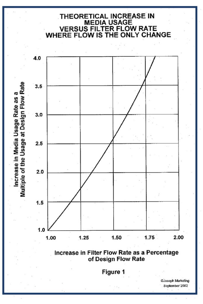
Figure 1 shows the operating characteristic of a filter’s media consumption at different levels of flow rate. The flow rate axis is plotted as a percent of increase over the designed flow rate when the filter was first selected. The origin is unity for media consumption at the designated parameters. However, as the flow rate increases, the rate of media usage jumps dramatically. For example, a 50 percent increase in liquid flow reflects an increase in media usage rate of 2.5 times. This is due to a change in the fluid flow rate only. There is no change in contaminant levels. This shows what “innocent” conditions such as unnecessary flushing on a machine can do to media operating costs.
Scenario 2: Planned increase in production machine up-time
Many times, during a production ramp-up, a media consumption rate was established in the early stages when the capacity of the line had not reached full production. Economics may be developed based on the operating cost at that point. Then, when production increases, it is erroneously expected that the media consumption rate will stay the same. This is not true.
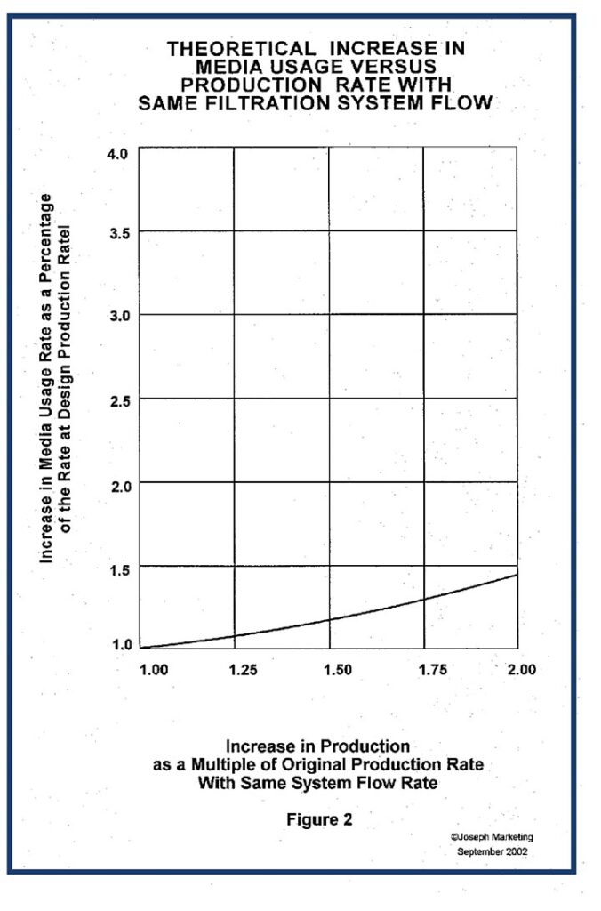
Figure 2 shows a math model based on actual production experience of how the disposable media usage climbs with respect to the production increase. In this case, the production ratio of an existing line is using the same flow rate but capitalizing on more up-time of the machines. For example, if an existing line does not change anything but increases its output by 50 percent during a production day, media usage will probably increase about 20 percent. This curve can be used as a rule of thumb. It must be recognized that other varying parameters could cause a different operating characteristic. At least the curve shows the correlation of more productivity on the same line and the media usage from the same filter.
It is noteworthy that the increase in media consumption, in this case, is far less than the increase due to fluid flow rate. The changes in fluid rates have a much greater impact on filter performance. Even if production doubles and flow rate stays the same, media consumption may only increase about 40 percent. Whereas, doubling the rate of fluid flow and with no increase in production the media usage rate could jump almost five times.
Scenario 3: Increase in production capacity
There is another scenario where a production plan adds more machines to a system, which will add both more flow and more contaminants. Often this is accomplished without the consideration of adding more filtration capability. Then the filter must handle not only the extra flow while serving the machines, but it must also carry the burden of the extra contaminants. The combination of Figures 1 and 2 (more flow and more contaminants) creates Figure 3, which reflects the change in media consumption.
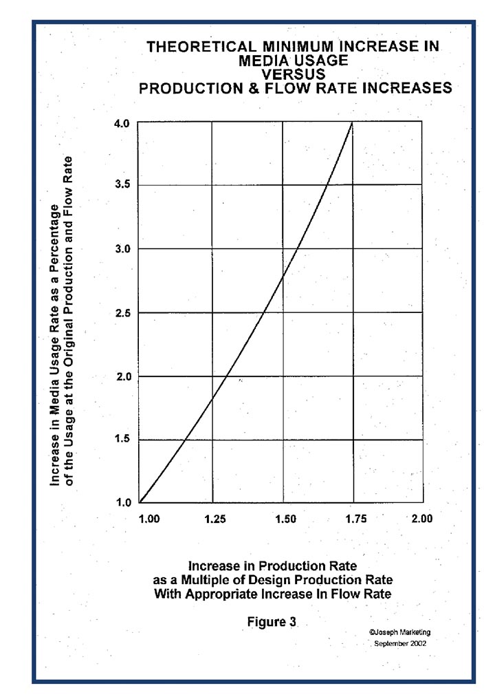
This change could be significant, and this should be factored into any justification analysis. For example, a 50 percent increase in production machines reflect a media consumption rate of 2.8 times the rate of the original production rate.
A revamped installation for more productivity may readily accept the higher cost of disposable media because it may save a considerable amount in equipment costs. However, if higher operating costs carry other burdens, such as disposal and environmental hazards, then there may be justification to adding supplementary equipment to the existing facility. The added equipment may not necessarily mean filters. Separators; i.e., centrifuges, magnetic units, or retention tanks, can be used to ease the burden on existing filters and allow them to operate near their original design. These could be positioned on-line or off-line as remote recovery systems.
In conclusion, the goal is to bring awareness that filter design/maintenance and media selection are not the only factors for media consumption. Issues on liquid flow rates, productivity, and filter set-up that could influence the rate of media use. Of all the reasons, the one that has the greatest influence is excessive flow through the filter regardless of the contamination levels.
If the flows are needlessly excessive, then they should be controlled.
A revamped installation for more productivity may readily accept the higher cost of disposable media because it may save a considerable amount in equipment costs.
If more machines are to be installed on the same line, then the extra media costs should be an entry in the economic analysis. Along with the extra media, there should be awareness that coolant life may be shorter and more frequent disposal and replenishment costs should be considered.
If the increase in operating costs due to adding more production to the same line are not economically justified, then the options of enhancing the system with supplementary devices may be viable. This could be particularly rewarding since the cost savings with less media and better fluid clarity could be a major contributor to the payback on the investment of additional clarification equipment.
Filtering Index Measurements
Calculations which show that when the flow through a given filter area is reduced to half, the media life is increased greater than 4 times. The following is using hydraulics and filter equivalence equations to support the statement that lowering the filter flow rate will extend filter life.
Caution this is a rough guide to attempt to predict filter media life for a liquid filtration applications. There are many factors involved which could influence the outcome differently.
The industry has claimed and shown that reducing the GPM per square foot will increase the cycle life of the media significantly. For example if the flow per square foot is reduced to half the flow and nothing else changes the cycle life of the media will be greater than four times the life it was before the reduction in flow.
The rough extrapolation can be determined using the filter equivalence equation.
Please remember this is a guide only. There are other factors involved as well as but following exercise may help understand the phenomenon.
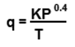
q is GPM per square foot
K is a constant
P is pressure differential across the filter media
T is relative cake thickness
“T” is the important factor here. Since the clarity was acceptable when the fluid went through a cake “T,” we will keep “T” value the same for the following points.
The calculations are solving for “P” with the same “T” value (for the same clarity). When a different flow rate is entered the different “P” reading is compared to the other “P” reading. The ratio reflects the time difference between media changes.
For example:
A vacuum filter with 10 GPM/sqft and a T of 15 has a pressure differential of 20 inches of water is the indexing set point. Say this indexed every 30 minutes. With the same T of 15, the flow at 5 GPM/sqft the pressure is 4 inches of water. If 20 inches of water is the indexing point the 5 GPM flow will take about 4 to 5 times longer to reach 20 inches or index every 120 to 150 minutes.
If the flow is increased to 20 GPM/sqft with T at 15, the pressure P would be 145 inches of water for P. Indexing is still at 20 inches of water. The 145 would be reached time between indexing would be 20 divide by 145. This shows the filter will index 0.14 the time at 10 GPM/sqft or every 4 minutes. Of course there are other factors such as compressibility, but this is a realistic guide.
Another way of looking at the flow to pressure ratio is to study the equation which is a derivation of the above equation. The hydraulic industry uses the following equation to calculate pressure drop across an orifice of known diameter at a specific flow.
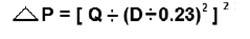
P = Pressure differential
Q = GPM
D = Orifice Diameter in inches (assumed media permeability)
It makes no difference what the value as long as the value is the same in both cases.
If we take Q as GPM/sqft and D as our “T” the following numbers are calculated.
When Q is 10 GPM and T is 0.25 the pressure is 70.5
When Q is 5 GPM and “T” is still 0.25, the pressure is 17.6
70.5 divided by 17.6 equals 4. So it can be safely stated that the pressure at 5 GPM climbs slower than the pressure at 10 GPM. If “T” is our clarity level the media will stay in the filter about 4 times longer.
— Jim Joseph, Joseph Marketing, ©August 30, 2012


